CSFlow

Baseline vs. CSFlow: Better image realism

Baseline

CSFlow (ours)

PixelGen-XXL/16 · text-to-image · 512×512

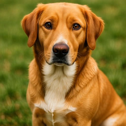Baseline

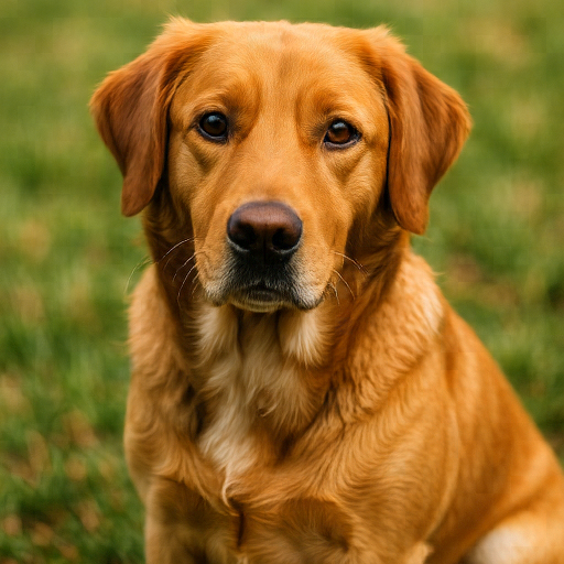CSFlow (ours)

PixelGen-XXL/16 · text-to-image · 512×512

TL;DR: Prioritize visually important generation stages

We introduce Contrast Sensitive Flow (CSFlow), a weighting scheme method for flow matching that prioritizes reconstruction of frequencies that are more important for the human eye. We combine two properties: first, that pixel-space image generation happens in a coarse-to-fine manner, where low frequencies are established before higher frequencies. Second, that the human eye is more sensitive to certain frequency bands. We redistribute several models' precision and capacity accordingly through a weighted inference and fine-tuning. The results: consistently better quantitative results (FID, GenEval) and images that look less "cartoonish" and oversmoothed, and achieve overall better realism.

Overview: Paper teaser

Abstract

Contrast Sensitivity Function: Test it with your own eyes

Depending on the viewing distance and displayed image size, your ability to see certain frequencies changes, which is exactly what CSF measures. This is a Campbell–Robson chart — spatial frequency increases left→right, contrast fades top→bottom. The dashed line is the predicted human visibility threshold: adjust the viewing distance and physical image width and watch it shift, computed from the real Barten CSF (Appendix A) and the visual-angle conversion in Appendix D.

Method

CSFlow is built on the forward process - iterative noising, and reverted over the time, to analyze how the frequency content changes during denoising. We built it in four steps: (1) measure how recoverable each image-frequency is when image is noised, (2) measure which image-frequencies are reconstructed between the noising-timesteps, (3) weight it by contrast sensitivity, (4) aggregate the resulting timestep weights.

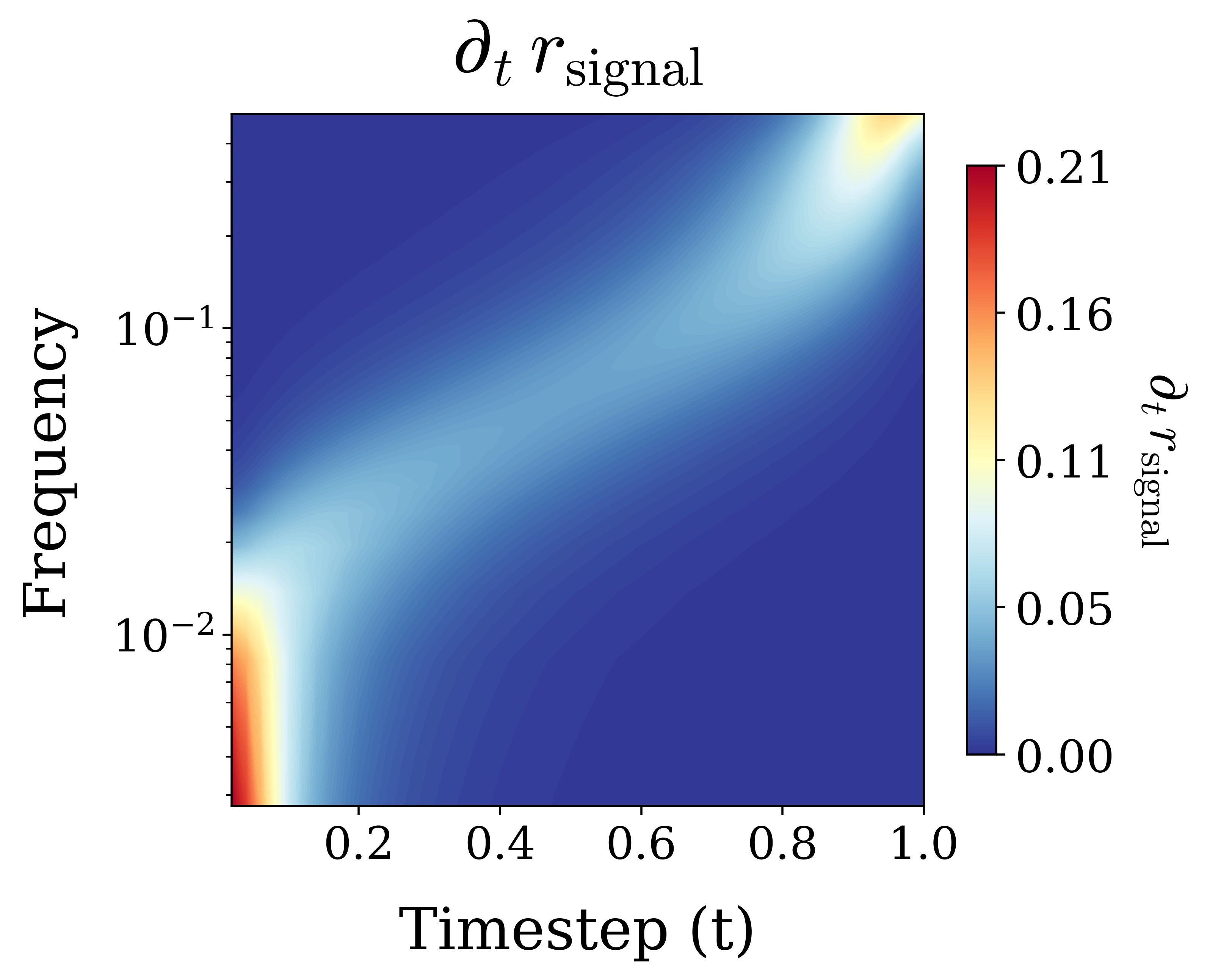
In the plots, we use a_t = t and b_t = 1-t, therefore, t = 0 corresponds to pure noise and t = 1 corresponds to the clean image.

01 — retained signal

How recoverable is each frequency?

For a noisy image at time t, we measure the fraction of each frequency's power that comes from the clean image rather than the noise. Near 0, all frequencies are noise-dominated; near 1, most are already settled and won't change much further with continued denoising.

r(f,t) = a_t² S_fa_t² S_f + b_t²

Closed-form retained signal — a normalized SNR per frequency, per timestep.

02 — ∂ₜ retained signal

Which frequencies are recovered at each step?

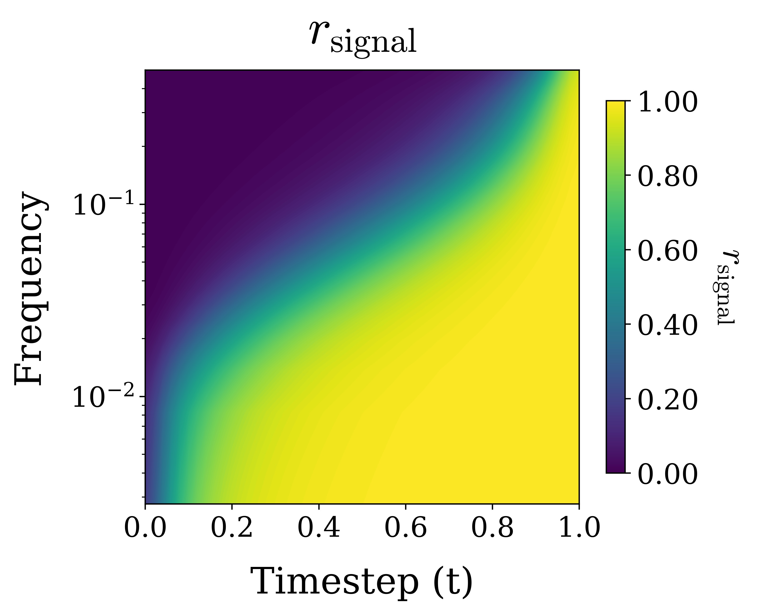
Retained signal alone only says how destroyed a frequency is — not what's changing. So we take the stepwise increase in retained signal over an interval [t, t+Δt] (or its continuous form, ∂ₜr). This is the amount of newly recoverable frequency content at that point in denoising — the measure of what the model is reconstructing right now.

∂ₜr(f,t,Δt) = r(f,t+Δt) − r(f,t)

Stepwise information gain — how much of frequency f becomes newly recoverable over [t, t+Δt].

03 — CSF-weighted ∂ₜ retained signal

Emphasize perceptually important frequencies

We combine the newly recoverable content at each step with the Contrast Sensitivity Function (CSF). This emphasizes frequency bands that are most visible to people, and therefore, timesteps which correspond to these frequencies.

s(f,t) = ∂ₜr(f,t) · CSF(f)

CSF-weighted newly recoverable frequency content.

04 — timestep weights

Allocate importance through weighting

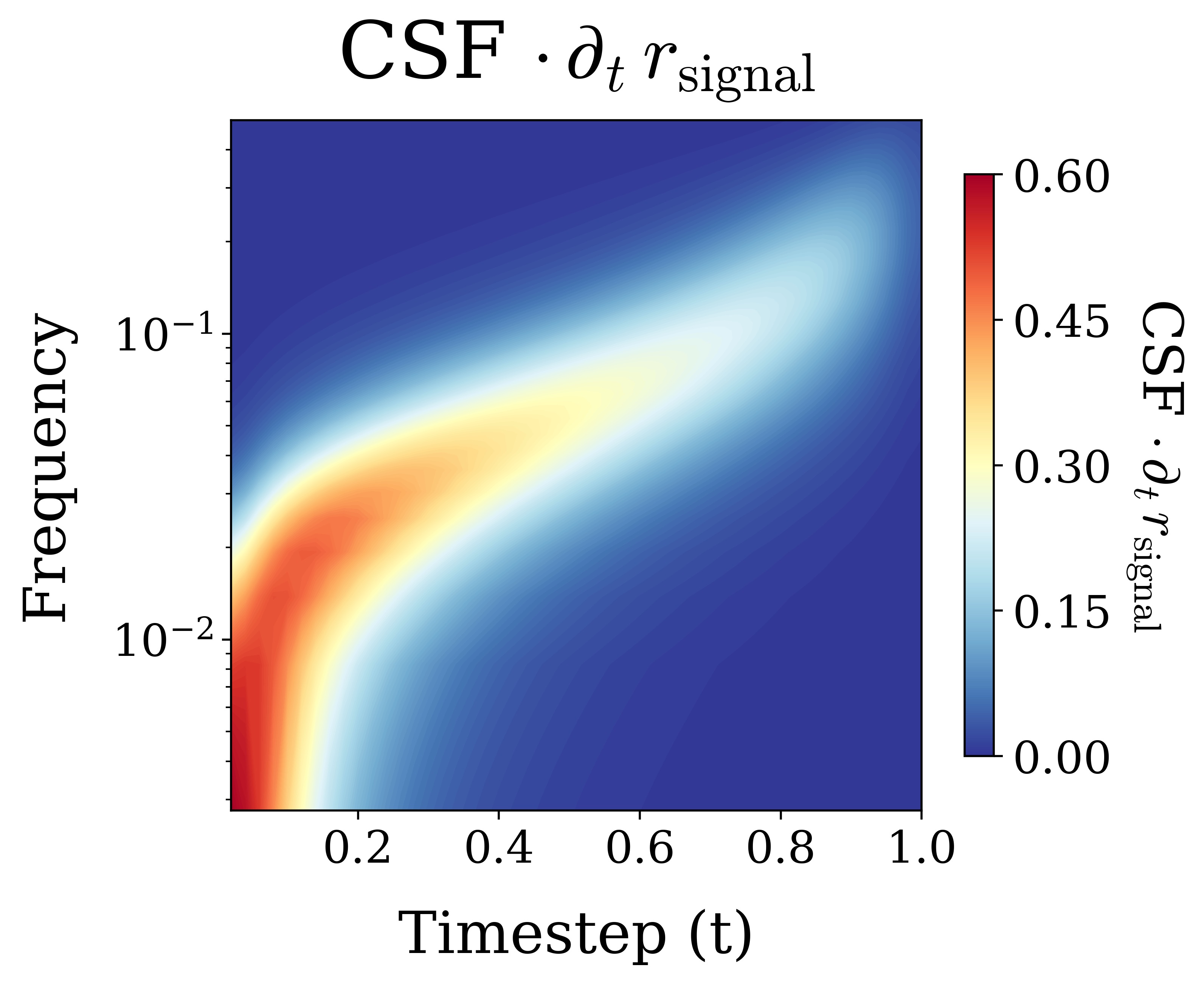
We aggregate the previous CSF-weighted importance across frequencies: each timestep is weighted by the average CSF of the frequencies newly recovered at that time.

w(t) ∝ ∫_Ω s(f,t) df ∫_Ω ∂ₜr(f,t) df

Final perceptual timestep weights.

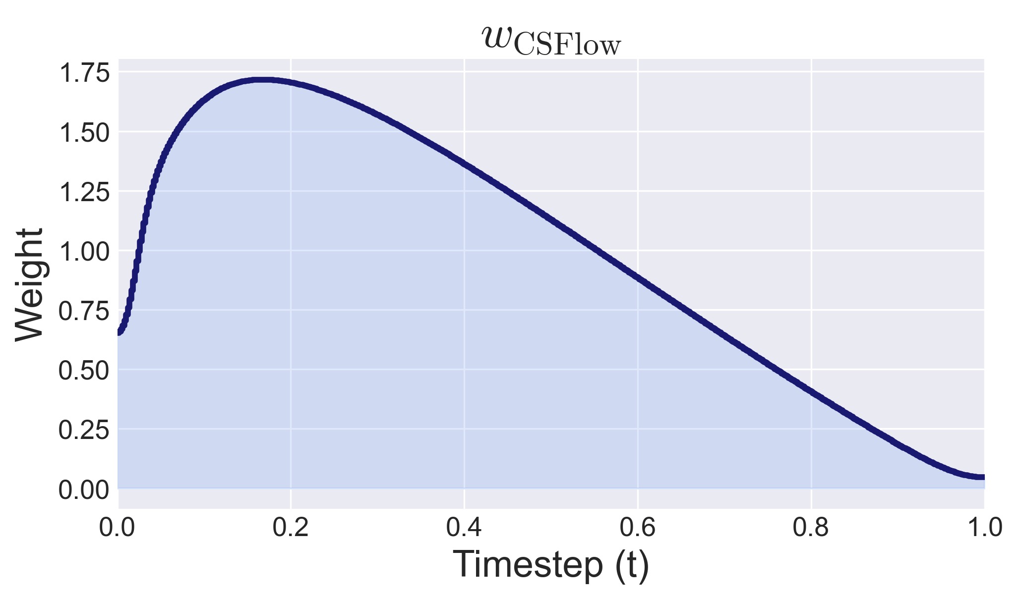
All plots use 50 uniform steps. At inference, the resulting weights reshape the timestep grid — we allocate smaller steps where perceptually important frequencies are reconstructed. In training, we bias which noise levels get sampled more often.

Results

We evaluate models with CSFlow and two other perceptually-driven weightings. We use PixelGen-XXL on text-to-image generation and report GenEval, and JiT-H, PixelREPA-H, and PixelGen-XL on class-to-image generation and report FID and Inception Score. Scores are averaged over five runs, with confidence interval set to 2 standard deviations. The displayed interpolation settings are the best-performing configurations for each method.

Interpolated with the base weights (individual best setup). All interpolation parameters are reported in the paper.

References

Cite this work: BibTeX

@misc{csflow2026,
      title={CSFlow: Aligning Flow Matching with Human Contrast Sensitivity},
      author={Malgorzata Galinska and Bart Pogodzinski and Jan Eric Lenssen},
      year={2026},
      url={https://arxiv.org/abs/2606.08833},
}